Data Science / Section 1 / Sprint 1 / 20.12.30
Top 25 Pandas tricks

Pandas DataFrame 활용
nbviewer.jupyter.org/github/justmarkham/pandas-videos/blob/master/top_25_pandas_tricks.ipynb
Jupyter Notebook Viewer
Now if you need a much larger DataFrame, the above method will require way too much typing. In that case, you can use NumPy's random.rand() function, tell it the number of rows and columns, and pass that to the DataFrame constructor:
nbviewer.jupyter.org
1) show installed verisons
pd.__version__ #단순버전확인
pd.show_versions() #버전외 기타정보 쫙
2) Creat an example DataFrame
df = pd.DataFrame({'col one':[100, 200], 'col two':[300, 400]})
pd.DataFrame(np.random.rand(4, 8))
pd.DataFrame(np.random.rand(4, 8), columns=list('abcdefgh'))
3)Rename columns
df = df.rename({'col one':'col_one', 'col two':'col_two'}, axis='columns')
df.columns = ['col_one', 'col_two']
df.columns = df.columns.str.replace(' ', '_')
df.add_prefix('X_')
df.add_suffix('_Y')
4)Reverse row order
drinks.head()
drinks.loc[::-1].head() #192행부터 상단에서 거꾸로 보여줌 (192, 191, 190, ,,, 3,2,1,0)
drinks.loc[::-1].reset_index(drop=True).head() #데이터셋은 뒤짚었지만 index 넘버링은 0,1,2,3,4로 시작
5)Reverse column order
drinks.loc[:, ::-1].head() #4번 명령어와 유사기능, 이번에는 열을 뒤에서부터 뒤짚어주는 기능
6)Select columns by data type
drinks.dtypes
country object
beer_servings int64
spirit_servings int64
wine_servings int64
total_litres_of_pure_alcohol float64
continent object
dtype: object
drinks.select_dtypes(include='number').head() #데이터중 숫자데이터만 셀렉 (int64 , float64)
drinks.select_dtypes(include='object').head()
drinks.select_dtypes(include=['number', 'object', 'category', 'datetime']).head()
drinks.select_dtypes(exclude='number').head()
7)Convert strings to numbers (어제 굉장히 고생했던 파트)
df = pd.DataFrame({'col_one':['1.1', '2.2', '3.3'],
'col_two':['4.4', '5.5', '6.6'],
'col_three':['7.7', '8.8', '-']})
df.astype({'col_one':'float', 'col_two':'float'}).dtypes
#하지만 세번째 col은 에러발생
# ' - ' 대쉬값은 float으로 변환시키지 못하기 때문
pd.to_numeric(df.col_three, errors='coerce') #에러발생하면 NaN으로 표기하라
pd.to_numeric(df.col_three, errors='coerce').fillna(0) #NaN자리에 0으로 채우려면
최종버전
df = df.apply(pd.to_numeric, errors='coerce').fillna(0)
한번에 전부 적용시키는 방법
8)Reduce DataFrame size
drinks.info(memory_usage='deep')
.
.
memory usage: 30.4 KB
##데이터가 커서 전체를 불러오는데 시간이 걸리거나 하는 경우 해결할수있는 방법
1) 필요한 열 값만 지정해준뒤 불러오기
cols = ['beer_servings', 'continent'] #원하는 컬럼 지정
small_drinks = pd.read_csv('http://bit.ly/drinksbycountry', usecols=cols) , #원하는 컬럼만 가져오기
small_drinks.info(memory_usage='deep')
.
.
memory usage: 13.6 KB
2)The second step is to convert any object columns containing categorical data to the category data type, which we specify with the "dtype" parameter:
dtypes = {'continent':'category'}
smaller_drinks = pd.read_csv('http://bit.ly/drinksbycountry', usecols=cols, dtype=dtypes) smaller_drinks.info(memory_usage='deep')
.
.
memory usage: 2.3 KB
9)Build a DataFrame from multiple files (row-wise)
#열은 같으나 행이 각각 다를때 열에 맞춰서 한번에 합쳐줄때
pd.read_csv('data/stocks1.csv')
pd.read_csv('data/stocks2.csv')
pd.read_csv('data/stocks3.csv')
from glob import glob
stock_files = sorted(glob('data/stocks*.csv')) stock_files
['data/stocks1.csv', 'data/stocks2.csv', 'data/stocks3.csv']
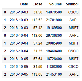
pd.concat((pd.read_csv(file) for file in stock_files))
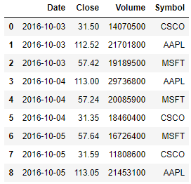
pd.concat((pd.read_csv(file) for file in stock_files), ignore_index=True)
10)Build a DataFrame from multiple files (column-wise)
#위와 동일한 방식
#이번에는 동일한 행에 열을 추가(합치는) 방법
pd.read_csv('data/drinks1.csv').head()
pd.read_csv('data/drinks2.csv').head()
drink_files = sorted(glob('data/drinks*.csv'))
pd.concat((pd.read_csv(file) for file in drink_files), axis='columns').head()
11)Create a DataFrame from the clipboard
#구글 스프레드시트 등에서 원하는 값을 선택, 복사한뒤
df = pd.read_clipboard()
#추천하지않는 접근방법이라고 함
12)Split a DataFrame into two random subsets
len(movies) #979
movies_1 = movies.sample(frac=0.75, random_state=1234)
movies_2 = movies.drop(movies_1.index)
len(movies_1) + len(movies_2)
movies_1.index.sort_values()
movies_2.index.sort_values()
13)Filter a DataFrame by multiple categories
movies.head()
movies.genre.unique()
array(['Crime', 'Action', 'Drama', 'Western', 'Adventure', 'Biography', 'Comedy', 'Animation', 'Mystery', 'Horror', 'Film-Noir', 'Sci-Fi', 'History', 'Thriller', 'Family', 'Fantasy'], dtype=object)
movies[(movies.genre == 'Action') |
(movies.genre == 'Drama') |
(movies.genre == 'Western')].head()
However,
you can actually rewrite this code more clearly by using the isin() method and passing it a list of genres
movies[movies.genre.isin(['Action', 'Drama', 'Western'])].head() #장르가 액션,드라마,웨스턴인것만
movies[~movies.genre.isin(['Action', 'Drama', 'Western'])].head() #장르가 액션,드라마,웨스턴 아닌것만
14)Filter a DataFrame by largest categories
counts = movies.genre.value_counts()
counts
Drama 278 Comedy 156 Action 136 Crime 124 Biography 77 Adventure 75 Animation 62 Horror 29 Mystery 16 Western 9 Sci-Fi 5 Thriller 5 Film-Noir 3 Family 2 Fantasy 1 History 1 Name: genre, dtype: int64
#장르별 숫자나열
counts.nlargest(3)
#높은 숫자 위에서부터 3개
counts.nlargest(3).index
Index(['Drama', 'Comedy', 'Action'], dtype='object')
#인덱스화
movies[movies.genre.isin(counts.nlargest(3).index)].head()
#isin() 안에 index 를 넣어줘야 인식후 제대로 작동하는구나
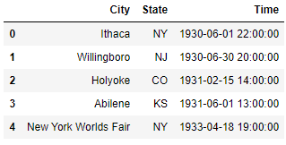
15)Handle missing values
ufo.head()
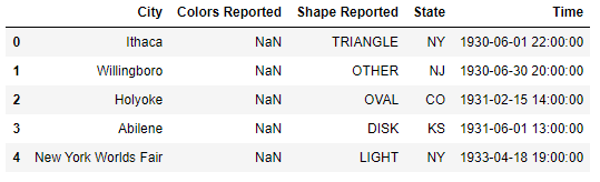
You'll notice that some of the values are missing.
To find out how many values are missing in each column, you can use the isna() method and then take the sum():
ufo.isna().sum()
City 25
Colors Reported 15359
Shape Reported 2644
State 0
Time 0
dtype: int64
isna() generated a DataFrame of True and False values,
and sum() converted all of the True values to 1 and added them up.
Similarly, you can find out the percentage of values that are missing by taking the mean() of isna():
ufo.isna().mean()
City 0.001371 (0.1%값이 missing value라는 뜻)
Colors Reported 0.842004 (84%값이 missing value라는 뜻)
Shape Reported 0.144948 (14%값이 missing value라는 뜻)
State 0.000000
Time 0.000000
dtype: float64
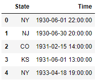
If you want to drop the columns that have any missing values, you can use the dropna() method:
ufo.dropna(axis='columns').head()
Or if you want to drop columns in which more than 10% of the values are missing,
you can set a threshold for dropna():
ufo.dropna(thresh=len(ufo)*0.9, axis='columns').head()
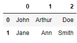
16)Split a string into multiple columns
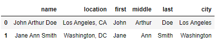
df = pd.DataFrame({'name':['John Arthur Doe', 'Jane Ann Smith'],
'location':['Los Angeles, CA', 'Washington, DC']})
df.name.str.split(' ', expand=True)
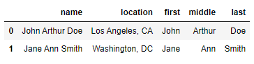
df[['first', 'middle', 'last']] = df.name.str.split(' ', expand=True) df
df.location.str.split(', ', expand=True)
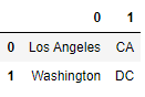
If we only cared about saving the city name in column 0,
we can just select that column and save it to the DataFrame:
df['city'] = df.location.str.split(', ', expand=True)[0]
17. Expand a Series of lists into a DataFrame
df = pd.DataFrame({'col_one':['a', 'b', 'c'], 'col_two':[[10, 40], [20, 50], [30, 60]]})
df_new = df.col_two.apply(pd.Series)
pd.concat([df, df_new], axis='columns')
18. Aggregate by multiple functions
orders.head(10)
orders[orders.order_id == 1].item_price.sum()
orders.groupby('order_id').item_price.sum().head()
orders.groupby('order_id').item_price.agg(['sum', 'count']).head()
19. Combine the output of an aggregation with a DataFrame
orders.head(10)
# create a new column listing the total price of each order?
orders.groupby('order_id').item_price.sum().head()
Out[82]:
sum() is an aggregation function(집계함수), which means that it returns a reduced version of the input data.
len(orders.groupby('order_id').item_price.sum())
1834
...is smaller than the input to the function:
len(orders.item_price)
4622
The solution is to use the transform() method,
which performs the same calculation but returns output data that is the same shape as the input data:
total_price = orders.groupby('order_id').item_price.transform('sum')
len(total_price)
4622
orders['total_price'] = total_price
orders.head(10)
orders['percent_of_total'] = orders.item_price / orders.total_price
orders.head(10)
20. Select a slice of rows and columns
데이터에서 특정 열또는 행만 보고싶을때
열범위값 또는 행범위값만 보고 싶을떄
titanic.head()
titanic.describe()
titanic.describe().loc['min':'max']
titanic.describe().loc['min':'max', 'Pclass':'Parch']
21. Reshape a MultiIndexed Series
titanic.Survived.mean() #서바이브드 된 열의 평균값
titanic.groupby('Sex').Survived.mean() #서바이브드 된 사람을 성별로 나눠서 낸 평균값
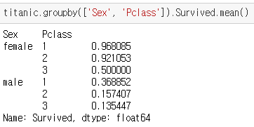
titanic.groupby(['Sex', 'Pclass']).Survived.mean() #서바이브드 된 사람을 성별과 Pclass로 나눠서 낸 평균값
This shows the survival rate for every combination of Sex and Passenger Class. It's stored as a MultiIndexed Series, meaning that it has multiple index levels to the left of the actual data.
It can be hard to read and interact with data in this format,
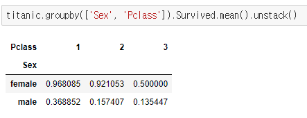
so it's often more convenient to reshape a MultiIndexed Series into a DataFrame by using the unstack() method:
다음과 같은 unstack() 방법을 사용하여 MultiIndexed Series를 DataFrame으로 변경하는 것이 더 편리합니다
22. Create a pivot table
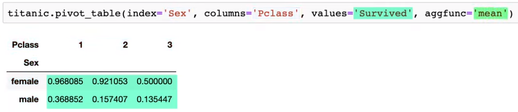
An added benefit of a pivot table is that you can easily add row and column totals by setting margins=True:
titanic.pivot_table(index='Sex', columns='Pclass', values='Survived', aggfunc='mean', margins=True)
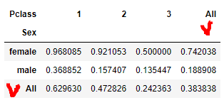
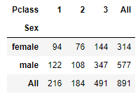
titanic.pivot_table(index='Sex', columns='Pclass', values='Survived', aggfunc='count', margins=True)
23. Convert continuous data into categorical data
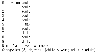
titanic.Age.head(10)
pd.cut(titanic.Age, bins=[0, 18, 25, 99], labels=['child', 'young adult', 'adult']).head(10)
### bins , labels 활용방법
# 0 ~ 18 까지는 'child'
# 18 ~ 25 까지는 'young adult'
# 25 ~ 99 까지는 'adult'
24. Change display options
titanic.head()
pd.set_option('display.float_format', '{:.2f}'.format) #소수점2까지만 표시하자
pd.reset_option('display.float_format')
25. Style a DataFrame
데이터프레임 색깔 , 표기 등
format_dict = {'Date':'{:%m/%d/%y}', 'Close':'${:.2f}', 'Volume':'{:,}'}
(stocks.style.format(format_dict)
.hide_index()
.highlight_min('Close', color='red')
.highlight_max('Close', color='lightgreen')
)
'AI월드 > ⚙️AI BOOTCAMP_Section 1' 카테고리의 다른 글
| Data Visulaize,plot,seaborn_Day4 (0) | 2021.01.03 |
|---|---|
| Data Manipulation,concat,merge,melt_Day3 (0) | 2020.12.30 |
| Feature Engineering,형변환_Day2(2) (0) | 2020.12.30 |
| Feature Engineering,데이터전처리,_Day2 (0) | 2020.12.29 |
| 시작,EDA,Data Science_Day1 (0) | 2020.12.28 |


댓글